What You Will Do:
- Learn how piecewise functions describe motion that changes direction or speed at different points in time on a position–time graph.
- Review key concepts: how the slope of each segment represents velocity, how the y-intercept sets the starting position, and how a flat segment represents the cart being stopped.
- Sketch your prediction of a piecewise motion pattern before collecting any data.
- Connect your MotionCart and roll it smoothly to match the shape of five piecewise position–time challenge graphs displayed in Desmos, capturing each result into your worksheet.
- Complete the Google Docs worksheet and submit it according to your teacher's instructions.
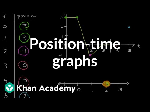
- To review position–time graph concepts before starting, click the video thumbnail below:
- Domain: the set of input values (time values, in this activity) for which a function is defined. On a position–time graph the full domain is the entire time axis from start to finish. In a piecewise function, each segment has its own restricted domain - a smaller interval of time during which that particular rule applies. For example, a segment might only be defined for $0 \le t \le 10$ seconds. Outside that interval the rule is not used; a different rule takes over.
- Watch this introduction to piecewise function:

- Piecewise function: a function built from two or more separate rules, each applied to its own restricted domain. Instead of one equation describing the entire graph, a piecewise function uses a different equation for each segment of time. In a position–time context, each piece represents a distinct phase of motion - perhaps the cart rolling forward, then stopping, then rolling backward. The full function is written by listing each rule alongside the interval of time it covers:
$$f(t) = \begin{cases} 10t & 0 \le t \le 4 \\ 40 & 4 < t \le 8 \\ -5t + 80 & 8 < t \le 16 \end{cases}$$This example describes motion that increases at 10 cm/s for the first 4 seconds to reach 40 cm, holds steady at 40 cm for 4 seconds, and then decreases at 5 cm/s back to zero by 16 seconds.
- Slope: on a position–time graph, the slope of a segment equals the cart's velocity - how fast it moves and in which direction.
- A steeper slope means the cart is moving faster.
- A positive slope means the cart is moving forward (position increasing).
- A negative slope means the cart is moving backward (position decreasing).
- A flat line (slope = 0) means the cart is stopped - this is a horizontal piece with a constant value on its restricted domain.
- Initial position: the position value where a segment begins on the graph. For the first segment this is the cart's starting position. For later segments, the initial position must match where the previous segment ended so the graph remains continuous. Note that a segment's initial position is not always the same as the y-intercept (b) in its equation y = mx + b.
- Continuity: in a piecewise motion graph each new segment must begin exactly where the previous one ended - the cart cannot jump to a different position. On the graph this means the endpoint of one piece and the starting point of the next must share the same position value, even though the slopes (velocities) on either side may differ.
- Click this link MotionCart -Activity 4 to open the worksheet in a new browser tab. Click Make a copy to save your version to your Google Drive.
-
Read the motion description below, then use your mouse to click and drag on the graph to sketch your prediction of what the position–time graph will look like.
The MotionCart starts at the origin (0 cm). It rolls forward and reaches 50 cm at 10 seconds. It remains at 50 cm for 5 seconds. It then rolls back and returns to the origin by 20 seconds. - If you need to start over, click Erase Drawing. When you are satisfied with your sketch, click Capture Drawing to copy the image to the clipboard and paste it into your worksheet.
- For detailed setup instructions, complete the Getting Started with MotionCart activity first.
- Turn on your MotionCart, connect it, and click Zero Position.
- Practice rolling the cart forward and back. Confirm that position increases when rolling forward and decreases when rolling back. If the sign is reversed, click Change Sign and roll again to confirm.
- Scroll down so the Desmos graph is fully visible. Practice starting a collection, rolling the cart, stopping the collection, and clearing the graph.
- In the Desmos expression list on the left, click the folder icon next to "Check your Prediction" to turn on the helper points. Notes in the expression list explain how to toggle items on and off.
- Zero the cart and position it at the starting point. Click Start Collection and roll the cart to match the helper points. Click Stop Collection when finished. Compare the resulting graph to the prediction sketch you made in "What Do You Think?" above. When you are satisfied, click Capture Graph and paste the result into your worksheet. Then click Clear Graph.
- Click the folder icon next to "Check your Prediction" to hide it, then click the folder icon next to Challenge 1 to display it.
- Zero the cart, click Start Collection, and roll to match the target graph. Click Stop Collection when finished, then click Capture Graph and paste the result into your worksheet. Repeat this process - Clear Graph, hide the completed challenge, display the next one - until you have completed and pasted all five challenge graphs into your worksheet.
- Paste your predicted drawing into your worksheet.
- Identify each segment's domain, calculate the slope and initial position, describe the motion, and write the piecewise function.
- Compare your prediction sketch to the graph you collected using the helper points and describe any differences.
- Discuss whether your collected graph is continuous and what a gap or jump would mean physically.
- Complete the five challenge graph-matches and paste each captured graph into your worksheet.
- When finished, submit your worksheet according to your teacher's directions.
- In the Desmos expression list, open the "Going Further - make your own" folder. Use the sliders to set the slope and y-intercept for each segment to create your own piecewise position-time graph. Then challenge a partner to replicate it with their cart.
- Click Hide Directions button in the upper left to give yourself more space. Start by checking your prediction using the helper points, then work through all five challenges. Capture and paste each graph into your worksheet before moving on to the next.