What You Will Do:

• Learn how the back-and-forth motion of your hand, carried by the MotionCart, can be modeled by sine and cosine functions.
• Review key concepts: periodic motion, amplitude, midline, period, frequency, and phase angle.
• Build a measured track with masking tape, a ruler, and two books, then sketch your prediction of the position-time graph before collecting any data.
• Collect position-time data as you roll the cart smoothly between the two books, then fit a sinusoidal model to your data in Desmos.
• Investigate how changing the amplitude, the frequency, and the starting point (phase angle) of your motion changes the graph and the equation.
• Complete the Google Docs worksheet and submit it according to your teacher's instructions.

Getting Ready:

• Position-time graph: a graph where the horizontal axis shows time $x$ (seconds) and the vertical axis shows the cart's position $y$ (centimeters from its zero point). In this activity the zero point is the center of your track, so positions on one side are positive and positions on the other side are negative. Your data appears in the Desmos table as $T$ (time), $S$ (position), and $V$ (velocity in cm/s, how fast and in which direction the cart is moving at each moment, calculated from the change in position).
• Periodic function: a function whose graph repeats the same pattern over and over. One complete repetition is called a cycle. Moving the cart from the center, out to one book, back past the center to the other book, and back to the center is one cycle.
• Sine function: $y = \sin(x)$. The graph starts on the midline at $x = 0$ and rises first toward its maximum.
• Cosine function: $y = \cos(x)$. The graph starts at its maximum at $x = 0$ and falls first toward the midline.
• General form: in this activity you will model your motion with
  $$y = A\sin\big(B(x - C)\big) + D$$
  Each of the four parameters changes the graph in a different way, described below.
• Amplitude $A$: the distance from the midline to a maximum (or minimum) of the graph. For your track, it is the distance from the center mark to either book.
• Period and $B$: the period $P$ is the time, in seconds, to complete one full cycle - on the graph, the horizontal distance from one peak to the next peak. $B$ sets the period: $P = \dfrac{2\pi}{B}$. A larger $B$ squeezes more cycles into the same time.
• Frequency $f$: the number of cycles completed each second, measured in hertz (Hz). Frequency is the reciprocal of the period, so $f = \dfrac{1}{P} = \dfrac{B}{2\pi}$. A faster back-and-forth rhythm means a higher frequency, a shorter period, and a larger $B$.
• Phase shift $C$ and phase angle: $C$ slides the graph right (positive $C$) or left (negative $C$) by $C$ seconds. The phase angle, $B \cdot C$, describes the same shift as an angle in radians - how far through a full $2\pi$ cycle the wave has been moved. A quarter-cycle shift is a phase angle of $\dfrac{\pi}{2} \approx 1.57$. A cosine graph is the same as a sine graph shifted left by a quarter cycle.
• Midline $D$: the horizontal line $y = D$ halfway between the maximum and minimum values of the graph. Because you zero the cart at the center tape mark, your midline should be close to $D = 0$.
• Before class, watch this short video to review the midline, amplitude, and period of sine and cosine graphs. Click the video thumbnail below:
  
  ×
• Click this link MotionCart - Activity 8 to open the worksheet in a new browser tab. Click Make a copy to save your version to your Google Drive.

Setting Up Your Track:

1. You will need masking tape, a ruler or meter stick, a pen or marker, and two books that can stand upright (hardcovers work best).
2. Clear a flat, straight stretch of table or floor at least 160 cm long.
3. Place a strip of masking tape across the middle of the space and label it 0. This is the zero point - the midline of your graph.
4. Choose an amplitude. Start with 50 cm. The amplitude may never be more than 70 cm, so every value you use in this activity must be 70 cm or less.
5. Use the ruler to measure the amplitude from the 0 mark in one direction and place a tape mark labeled +A. Measure the same distance in the other direction and place a tape mark labeled -A. Check that both marks are exactly the same distance from 0 - this is what makes the motion balanced about the midline.
6. Place the cart on the track with the USB-C port (the front of the cart) facing the +A mark. You will always line up the front edge of the cart with a mark.
7. Roll the cart until its front edge is on the +A mark and stand a book upright against the front of the cart. Then roll the cart until its front edge is on the -A mark and stand the second book upright against the back of the cart. The books act as gentle stops, so each swing turns around at the same place every time, which makes your motion much easier to repeat and your data more consistent.

What Do You Think?

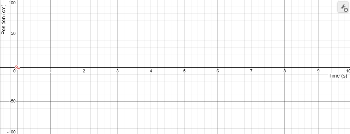
1. Read the motion description below, then use your mouse to click and drag on the graph to sketch your prediction of what the position-time graph will look like.
   The books are placed 50 cm on either side of the 0 mark. The MotionCart starts at the 0 mark and is moved smoothly toward the +A book first. It slows down as it reaches each book, turns around, and moves fastest as it passes the 0 mark. It completes one full cycle - out to +A, back to -A, and back to 0 - every 4 seconds, and keeps going for 10 seconds.
2. If you need to start over, click Erase Drawing. When you are satisfied with your sketch, click Capture Drawing to copy the image to the clipboard and paste it into your worksheet.
Capture Drawing Erase Drawing

3. In your worksheet, answer: how many complete cycles should appear in 10 seconds? What should the highest and lowest positions on your graph be? How would your sketch change if the cart started against the +A book instead of at the 0 mark?

Using Your MotionCart:

1. For detailed setup instructions, complete the Getting Started with MotionCart activity first.
2. Turn on your MotionCart and connect it. Place the cart with its front edge on the 0 mark, facing the +A book, and click Zero Position.
3. Roll the cart toward the +A book and confirm that the position increases and reads close to your amplitude when the cart touches the book. If the position decreases instead, click Change Sign and check again. Roll to the -A book and confirm the position reads close to the negative of your amplitude.
4. Practice the motion a few times before collecting. Hold the cart lightly with your fingertips and move it back and forth between the books in a smooth, steady rhythm. Slow down as you approach each book, just touch it, and move fastest as you pass the 0 mark - like a swinging pendulum. Do not pause at the books.
5. To keep a steady rhythm, have a partner count out loud or use a metronome app. For a 4-second period, touch the +A book on count 1 and the -A book on count 3 of a steady one-per-second count.
6. Return the cart to the 0 mark, hold it still, and click Zero Position again so the center reads 0 cm.
7. Scroll down so the Desmos graph is fully visible before you start collecting.
8. Click Start Collection. The button will turn yellow and display "Waiting for Motion..." - the system is watching for the cart to start moving, but hasn't recorded anything yet.
9. Begin moving the cart toward the +A book and keep your rhythm going. As soon as the cart moves, collection begins automatically from time zero and the button turns red.
10. Collection stops automatically at 10 seconds (the right edge of the graph), when the cart is held still for two seconds, or when you click Stop Collection.
11. Use Clear Graph to reset and try again. Repeat until you have a clean, even-looking run.
12. Once you have a clean run, move on to Analyzing Your Data below to model it.

Analyzing Your Data:

• In the Desmos expression list below, find the Sine Model folder, click the circle to its left to show the model, and then click the triangle to expand the folder and reveal the $A$, $B$, $C$, and $D$ sliders.
• Drag the sliders to adjust the model $y = A\sin\big(B(x - C)\big) + D$ until the curve fits your collected data as closely as possible. A good order is: $D$ to center the curve on the data, $A$ to match the height of the peaks, $B$ to match how often the peaks repeat, and finally $C$ to slide the curve left or right onto the data.
• Record the values of $A$, $B$, $C$, and $D$ in your worksheet. How does your fitted $A$ compare to the distance you measured with the ruler? Is $D$ close to 0? If not, what does that tell you about where you zeroed the cart?
• Find the period directly from your data by reading the time of two neighboring peaks and subtracting. Then calculate the period from your model using $P = \dfrac{2\pi}{B}$. Do they agree? Use the period to find the frequency $f = \dfrac{1}{P}$.
• Compare your prediction sketch to your fitted model. How closely does the shape, height, and number of cycles in your prediction match? Where are the biggest differences, and what does that tell you about your prediction?
• What part of the motion does your hand control that sets $A$? What part sets $B$?
• Click the Capture Graph button to copy your graph and then switch to the browser tab with your Google Docs worksheet and paste it into the doc.
• Click Clear Graph, then continue on to Investigating Amplitude, Frequency, and Phase Angle below.

Investigating Amplitude, Frequency, and Phase Angle:

1. Amplitude - keep the same 4-second rhythm, but move the books so the amplitude is 30 cm, then 70 cm. Re-measure and re-tape the +A and -A marks each time. Collect a run for each, fit the Sine Model, and record $A$ and $B$.
   • Which slider changed and which stayed about the same? Explain why using what your hand did differently.
2. Frequency - set the amplitude back to 50 cm. Collect one run with a slow rhythm (one cycle every 5 seconds) and one with a fast rhythm (one cycle every 2 seconds). Fit the Sine Model to each and record $B$.
   • For each run, calculate the period $P = \dfrac{2\pi}{B}$ and the frequency $f = \dfrac{B}{2\pi}$. How did $B$ and $f$ change when you moved faster? Check that $f \cdot P \approx 1$ for each run.
3. Phase angle - with a 50 cm amplitude and a 4-second rhythm, click Zero Position with the cart at the 0 mark, then roll the cart until it rests against the +A book. Click Start Collection and begin moving toward the 0 mark. Now your motion starts at the maximum instead of the midline.
   • Fit the Sine Model to this run. What value of $C$ did you need? Compare it to one quarter of your period, $\dfrac{P}{4}$. Which direction did the graph shift?
   • Calculate the phase angle $B \cdot C$. How close is it to $\pm\dfrac{\pi}{2} \approx \pm 1.57$?
   • Turn off the Sine Model folder and turn on the Cosine Model folder, $y = A\cos\big(B(x - C)\big) + D$. What value of $C$ fits this run now? Explain why the same motion can be written as either a sine or a cosine function.
4. Capture a graph from each investigation and paste it into your worksheet with your answers.

Going Further:

• Start the cart against the -A book and begin moving toward the 0 mark. Predict $C$ and the phase angle for the Sine Model before you collect, then test your prediction.
• Start the cart at the 0 mark but move toward the -A book first. What value of $C$ fits? How else could you write this function by changing the sign of $A$ instead?
• Zero the cart at the 0 mark, but set up your books so the motion is centered 20 cm to one side. Which parameter changes, and by how much?
• Velocity is periodic too. Turn on the $V$ column in the data table and compare its graph to your position graph. Where is the velocity largest, and where is it zero? Fit a sine model to the velocity data: how do its $B$ and $C$ compare to your position model's? The velocity graph is shifted a quarter cycle ahead of position - the same shift that turns a sine into a cosine.

Let's Go:

• Click Hide Directions to give yourself more space, then complete the activity and your worksheet.