Pressure Activity 1

What You Will Do:

Watch the Khan Academy video: "Boyle's Law" and review related concepts.
Explore how the microscopic impacts of gas particles account for the pressure of a gas.
Collect pressure data in the Desmos Graphing Calculator for decreasing volume of a hand syringe.
Build a mathematical model of the relationship between volume and pressure.
Complete the Google Docs worksheet: "Boyle's Law" and turn it in according to your teacher's directions.

Getting Ready:

Gas particles: tiny molecules that move in constant, random motion.
Pressure: the total force from countless microscopic impacts of gas particles hitting the walls of a container.
Volume: the amount of space available for gas particles to move around in.
Collision rate: how often gas particles strike the container walls; higher collision rates mean higher pressure.
Click to watch this Khan Academy video to learn more about these concepts.

Click this link Boyle’s Law Worksheet to open the worksheet. If your class uses Google Classroom, open the worksheet from your assignment. If not, click the link above, choose Make a copy, complete your work, and turn it in the usual way.
Click the Show Directions button in the upper-right corner to learn how to collect data for this activity.

What Do You Think?

Observe the motion of the particles in the simulation below and how they impact the inside of the syringe. Imagine a handful of tiny pebbles hitting your hand in a similar way. What would you feel from all of those impacts?
Click the syringe's minus (-) button to reduce the volume the particles move within and observe the effect on the impact rate of the particles.
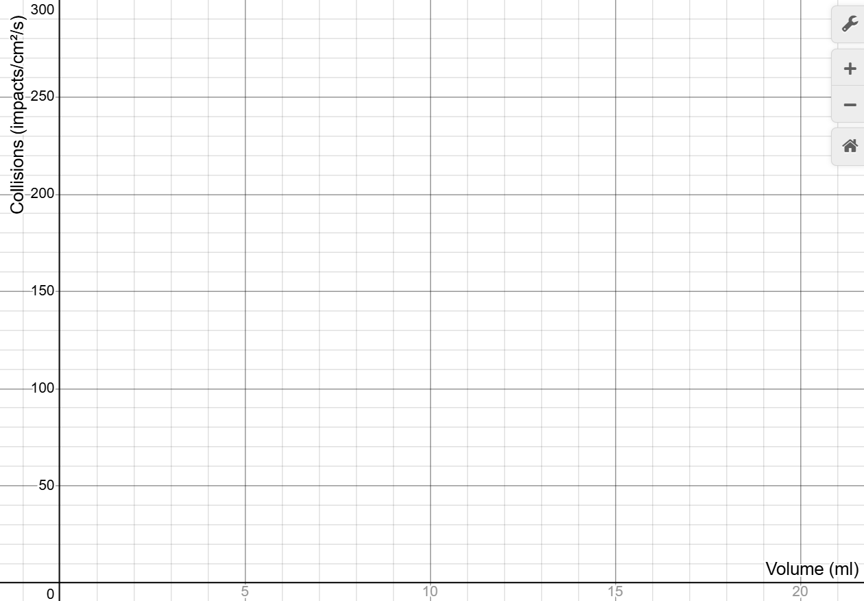
Repeat reducing the volume by 2 mL and allowing the impact rate to settle. Imagine what a graph with volume on the horizontal axis and impact rate on the vertical axis would look like.

20 mL Collisions = 0.00 Impacts/cm²/s

Use your mouse to click and drag on the graph to draw your prediction. If you need to start over, click Erase Drawing. When you are satisfied, click Capture Drawing to copy the image to the clipboard and paste it into the Boyle's Law worksheet and answer the related questions.

Directions:

Use a USB-C cable to plug the Observe pressure sensor into your computer's USB port.
Click the Connect Sensor button to activate the sensor.
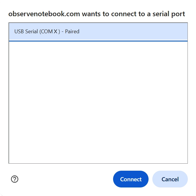
Select the USB serial port (COM X). The X value varies by computer and is not important. Then click the blue Connect button in the pop-up window. The status will change to ready.

Adjust the plunger of the syringe to exactly 20 mL and attach the syringe to your pressure sensor. Notice the pressure reading in units of kilopascals (kPa) above the graph. Pressing the plunger down to reduce the volume causes the pressure to increase.
Add measurements one at a time by pressing the Add Point button. When pressed, you are prompted for the x-value for the corresponding y measurement. Your first point should be 20 mL. Next, reduce the volume by 2 mL and add another point. Continue reducing the volume by 2 mL and adding points until a volume of 6 mL.
Clear Graph resets; Capture Graph copies an image of the graph to the clipboard; Export/Import saves or opens a CSV data file.
Click the small gray triangle to the left of the data table to view the sensor data (V and P) in the table.
Click the Show Instructions button in the upper right to continue.

Data Collection

(0, —)

Analyzing Your Data:

Based on your experience from the simulation, do you think the relationship between pressure and volume is direct or indirect? How would you mathematically express these two relationships?
Build your mathematical model using Least-squares regression.
- Press the + button in the upper left of the Desmos table and select Expression.
- Build a model that predicts the pressure (P) for a given volume (V). Use the tilde symbol to apply the Desmos regression feature.
- If you think a direct relationship is best, enter:
- Otherwise, if you think an indirect relationship is best, enter:
Test your model by predicting the value of pressure when the volume is 25 mL. Since 25 is larger than any value in the data set, this process is known as extrapolation.
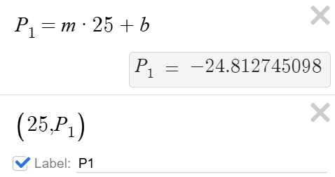
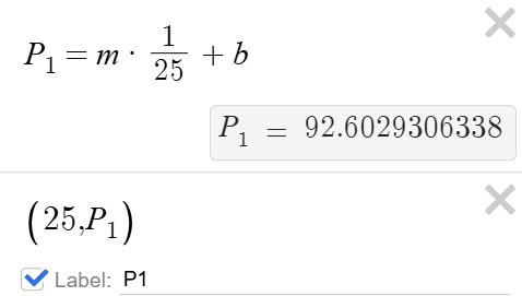
Use the slope (m) and y-intercept (b) from your regression equation to make a prediction by substituting 25 mL into the model.
Plot the predicted point on your graph and judge how well the point fits the model.
For a linear model, enter:

Going Further:

Try repeating the above steps to test an interpolated prediction using your regression model.
Use Desmos to display the residuals (click the plot icon under “RESIDUALS”) for your model. What patterns do you notice? What does this tell you about how well the model fits the data?
Try Activity 3: Temperature and Molecular Motion to learn more about statistical models and molecular motion.

Activity 1: Boyle's Law